Nuclear astrophysics with γ beams
Lecture notes for the 13th European Summer School on Experimental Nuclear Astrophysics
The origin of p-nuclei, an open question for nuclear astrophysics
A small group of around 35 stable neutron–deficient nuclei with A $\geq$ 74 between selenium (Se) and mercury (Hg) cannot be produced by the two main neutron-capture processes (s- and r-process). These are referred to as p-nuclei and their origin is a long-standing puzzle.
The fact that a distinct process produces these isotopes had been already identified from the early days of our field by both Cameron
For this reason their solar abundances
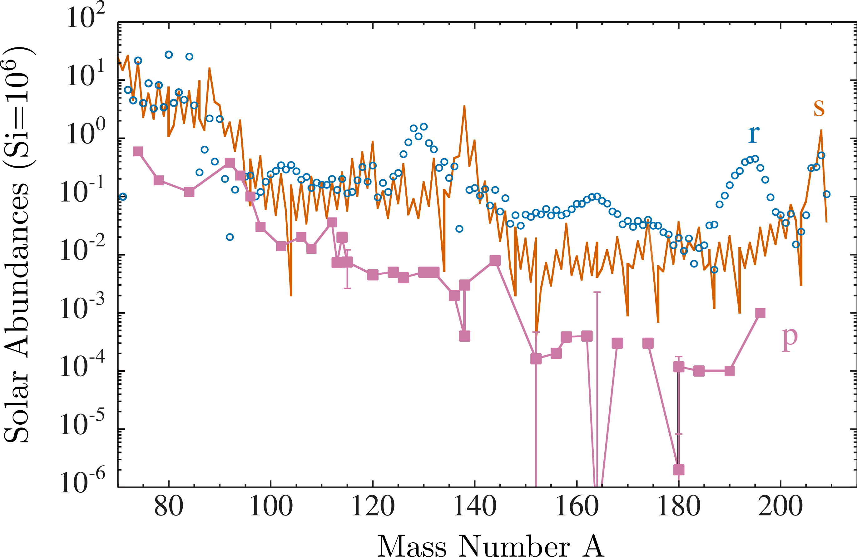
It is generally accepted that the p-nuclei in the solar system have been produced by more than one processes; however their synthesis mechanism is commonly referred to as p-process. In the following we shall focus on one scenario operating in massive stars called the $\gamma$-process.
How to produce the p-nuclei
Core-collapse supernovae (ccSNe) explosions are the last evolutionary stage of massive stars with $M \sim 8~M_{\odot}$.
During the explosion, the shock-wave that propagates towards the outer layers of the star induces the production of p-nuclei through photodisintegration reactions.
For this reason, this scenario is referred to as $\gamma$-process
The $\gamma$ process network is vast, involving more than 2,000 nuclei (most of them radioactive) with >20,000 reactions!
The initial seeds are isotopes produced previously during the s-process in the AGB phase of the massive star, or even r-process isotopes that polluted the nebula that produced the massive star. For this reason, knowing this seed distribution accurately (and the neutron-producing reactions!) is a key uncertainty in $\gamma$-process modeling.
See lectures by M. Busso and M. Pignatari
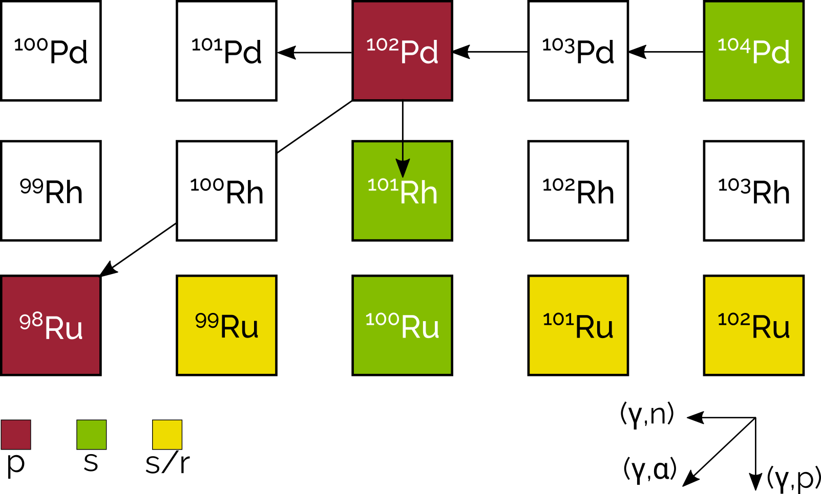
As we can see from the top figure, the main drivers of the $\gamma$-process are $(\gamma,n)$, $(\gamma,p)$ and $(\gamma,\alpha)$ reactions. Of importance are the branching points, where the flow moves to lower mass isotopes. In this cases, the competition between $(\gamma,n)$ and the other two channels can change the reaction flow, and eventually the final p-nuclei abundances.
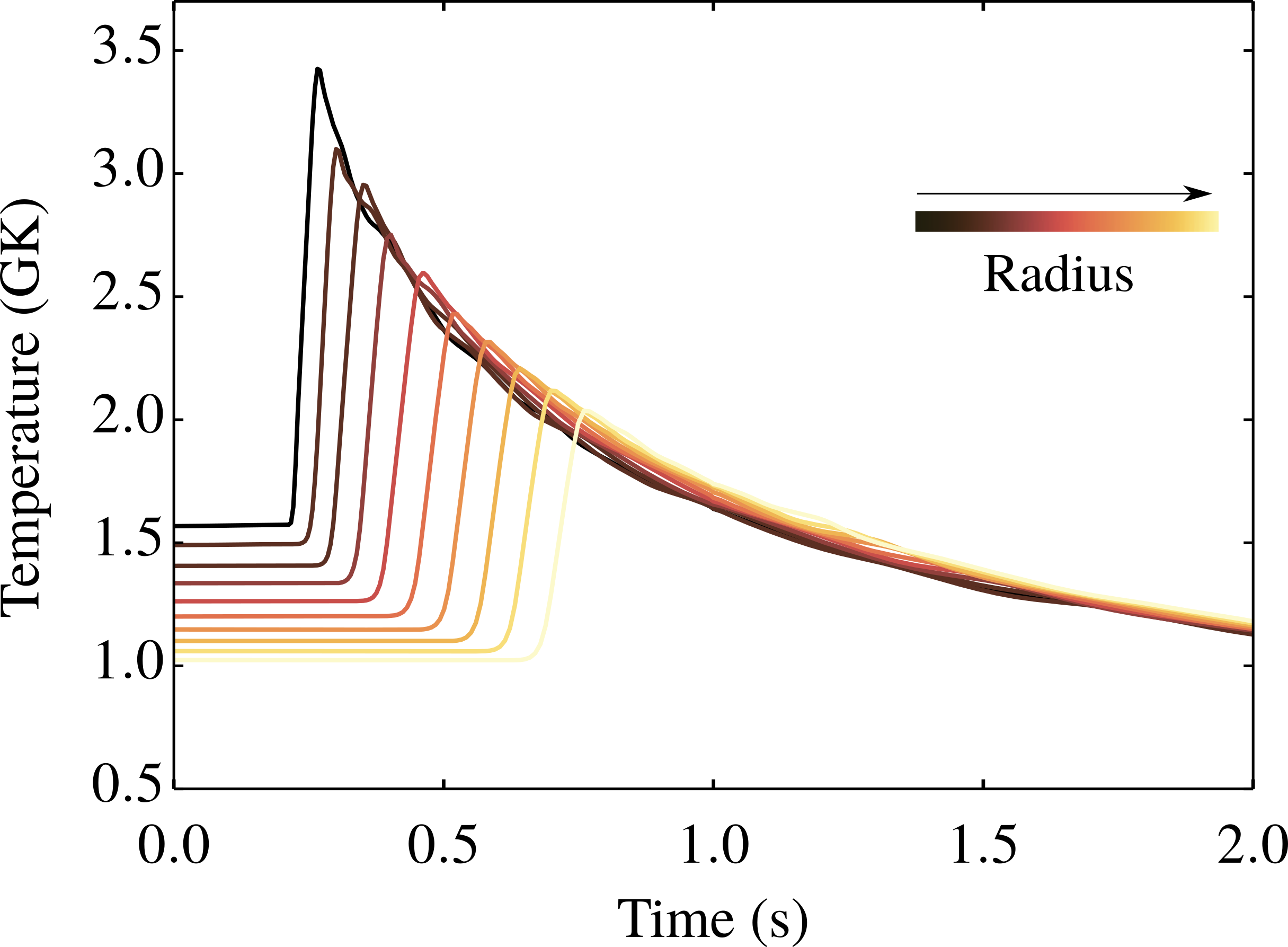
In the $\gamma$–process each mass region is produced at a different peak temperature: intermediate mass p–nuclei (A~ 92–136) are produced at $T \sim 2.5 − 3$ GK while the heavy p–nuclei (A > 140) at $T < 2.5$ GK. For this reason it is important to have a good understanding of the temperature and density profiles of the shock wave as it propagates through the outer layers of the star, which is still a major uncertainty in $\gamma$-process modeling.
More recently, C-O shell mergers in the pre-explosion phase have been proposed as a candidate for the production of the p-nuclei
ccSNe are also hosts for two additional processes that produce a small subset of the p-nuclei via reactions that involve neutrinos. The $\nu$-process has been shown to produce some rare species, such as $^{152}$Gd, $^{164}$Er, $^{180}$Ta
Another viable astrophysical environment for the production of the p-nuclei is thermonuclear supernovae (type Ia).
In this explosion, a white dwarf is disrupted when its mass surpasses the Chandrasekhar limit, while accreting material from a companion star.
The production of p-nuclei in type Ia supernovae has been studied in detail in the literature and it strongly depends on the initial composition of the white dwarf
Accreting neutron stars via the rp-process have also been shown to produce p-nuclei, via proton captures instead of photon disintegrations, however it is not clear if they can contribute to the galactic chemical evolution due to extremely large escape velocities from a neutron star surface that hinder any ejection of material into the interstellar medium
Despite our ability to reproduce most of the p-nuclei abundances of the solar system to within a factor of 2, there are still a few cases where the $\gamma$-process fails to reproduce in sufficient amounts; notable examples include the light $^{92,94}$Mo, $^{96,98}$Ru, $^{113}$In, $^{115}$Sn, $^{138}$La, $^{180}$Ta that most likely have contributions from other processes
The nuclear physics of the $\gamma$-process
The Hauser-Feshbach (HF) statistical model
Given the vast size of the $\gamma$-process network (>2,000 nuclei), we cannot directly measure all the relevant reactions at the temperatures of interest. Thankfully, theoretical calculations bridge this gap. The Hauser-Feshbach (HF) model is the standard approach for calculating photodisintegration (and radiative capture) cross sections in the intermediate- to heavy-mass regime where level densities are high.
In a photodisintegration reaction, a $\gamma$-ray is absorbed by a nucleus, forming a compound nucleus in an excited state. The compound nucleus then decays through one or more exit channels (neutron, proton, alpha emission, or $\gamma$-ray emission) independently of how it was formed. The assumption that the compound nucleus “forgets” its formation mechanism underlies the HF model.
The HF model expresses the cross section as:
\begin{equation} \sigma(E) = \pi \hbar^2 \sum_{J,\pi} g(J^\pi) \frac{T_\mathrm{in}(E) T_\mathrm{out}(E)}{T_\mathrm{tot}(E)} \end{equation}
where:
- $g(J^\pi)$ is the density of states (or transmission coefficient weighting) for angular momentum $J$ and parity $\pi$
- $T_\mathrm{in}(E)$ is the transmission coefficient for the entrance channel (photon absorption)
- $T_\mathrm{tot}(E)$ is the total transmission (sum over all competing channels, e.g. proton, neutron and alpha)
Each output is weighted by its own transmission coefficient, which depends on the nuclear level density (NLD) and $\gamma$-ray strength function ($\gamma$SF), which are the three main sources of uncertainty in HF predictions:
-
Optical-model potential (OMP): The complex potential describing nucleon scattering in the nucleus. Different parameterizations (e.g., Koning–Delaroche, RIPL-3) can differ by factors of 2–3 in transmission coefficients, especially for neutrons.
-
$\gamma$-ray strength function ($\gamma$SF): The probability for a nucleus to emit (or absorb) a photon at a given energy. The $\gamma$SF is constrained by photon scattering experiments (NRF), but extrapolation to higher energies carries large uncertainties. Different models (e.g., Lorentzian, Brink-Axel, microscopic) can differ significantly.
-
Nuclear level density (NLD): The number of available quantum states per unit energy. For low excitation energies, individual levels are resolved; at higher energies (where the $\gamma$-process operates), the density grows rapidly. The NLD is often parameterized by Fermi-gas models, with parameters that differ between codes.
As you can imagine, the uncertainties in these three ingredients propagate to the predicted thermonuclear reaction rates, and as a result to the final $\gamma$-process abundance predictions through nucleosynthesis calculations.
A factor of 2 error in a single reaction rate can alter the final p-nucleus abundances by orders of magnitude at branching points
See lecture by A. Tsantiri
Many codes can perform these calculations, with the most well-known in our community being:
- TALYS
- NON-SMOKER (SMARAGD)
- EMPIRE
For the first two, you can access database results for different reactions in NON-SMOKERweb and TALYS world.
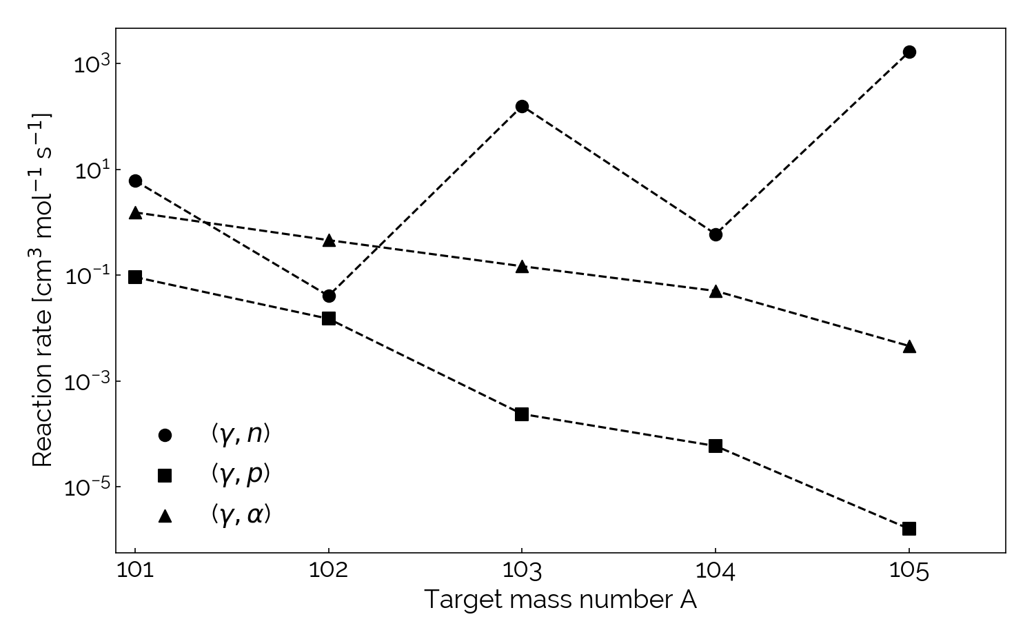
Let us now explore how we can use these theoretical nuclear physics calculations to study the $\gamma$-process. In the following example, we have plotted the reaction rates for the three competing reaction channels, $(\gamma,n)$, $(\gamma,p)$, and $(\gamma,\alpha)$ in the palladium isotopic hain. The branching from one isotopic line to the next happens when the proton or the alpha channel is stronger than the neutron. Here the branching happens in $^{102}$Pd which is the nucleus we will study in more detail in the following. Note that we haven’t included any uncertainties in these calculations, meaning that the branching point might change if we change the nuclear physics input, which is why experiments are so important to constrain the models.
Detailed balance- Connecting forward and reverse reactions
The detailed balance principle allows us to extract photodisintegration cross sections from radiative capture data. For a reaction $A + a \leftrightarrow B + b$, detailed balance relates the forward reaction rate to the reverse:
\begin{equation}\label{eq:detailed_balance} \langle \sigma v \rangle_{(p,\gamma)} = \frac{(2J_B+1)}{(2J_A+1)} \frac{E_{\gamma}^2}{(m_pc^2 kT)^{3/2}}e^{-Q/(kT)} \langle \sigma v\rangle_{(\gamma, p)} \end{equation}
Here, $Q = (m_A + m_p - m_B - m_\gamma)c^2$ is the Q-value (negative for endothermic reactions). The temperature dependence $T^{-3/2}$ reflects the thermal distribution of particles in the plasma (Maxwell-Boltzmann). The spin factors $(2J+1)$ account for the different quantum states available in each channel.
At higher temperatures, the exponential factor $e^{-Q/(kT)}$ grows, making the photodisintegration rate larger compared to radiative capture. This is why the $\gamma$-process is efficient in core-collapse supernovae, where temperatures exceed GK!
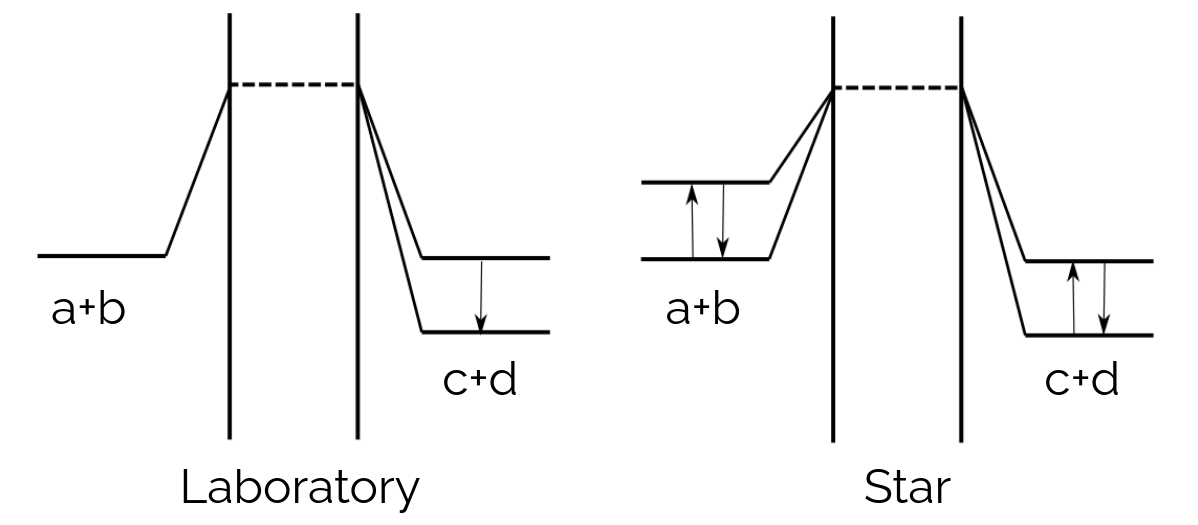
Stellar enhancement and partition functions
In the astrophysical environment, nuclei are not confined to their ground states. Thermal excitation populates excited levels, and the effective cross section seen in a stellar plasma depends on:
-
Partition function: The fraction of nuclei in excited states is given by the partition function: \begin{equation} G(T) = \sum_i (2J_i+1) e^{-E_i/(kT)} \end{equation} where the sum runs over all accessible excited levels. At low $T$, only the ground state contributes; at high $T$, many levels are populated.
-
Stellar enhancement factor: The ratio of the stellar rate to the ground-state rate is approximately: \begin{equation} \frac{\langle \sigma v \rangle_\star}{\langle \sigma v \rangle_{g.s.}} \approx \frac{\sum_i (2J_i+1) \sigma_i(T) e^{-E_i/(kT)}}{(2J_{g.s.}+1)\sigma_{g.s.}(T)} \end{equation}
Different excited states have different spins and resonance strengths. A measurement targeting only the ground state can miss significant contributions from excited levels. This is particularly important near energy thresholds, where ground-state contributions might be suppressed but excited-state contributions could be substantial
For more details on how to calculate partition functions and apply them to astrophysical rates, see
Why $\gamma$-beam experiments matter
As we have discussed already, the $\gamma$-process network is vast (>2,000 nuclei, >20,000 reactions), making it impossible to measure all reaction rates directly. For photodisintegration reactions (the reverse of radiative capture), direct measurements are particularly challenging, but very important.
See lectures by G. Gyürky and A. Tsantiri
Typically, we can use the time-reversal symmetry of nuclear interactions to get the photodisintegration rates. If we measure the forward reaction (e.g., $p + ^{101}\mathrm{Rh} \rightarrow \gamma + ^{102}\mathrm{Pd}$)
In stellar environments, nuclei exist in excited states due to the high temperatures. The competition between different exit channels—$(\gamma,n)$ vs. $(\gamma,p)$ vs. $(\gamma,\alpha)$—depends sensitively on where the compound nucleus has strength (resonances). Monoenergetic $\gamma$-beams allow us to scan through these resonances systematically.
The HF model relies on inputs like the optical-model potential, $\gamma$-ray strength function, and nuclear level density. By measuring cross sections at energies relevant to the $\gamma$-process, we can constrain these inputs and reduce uncertainties in theoretical predictions.
$\gamma$-beam experiments DO NOT provide the full stellar rate, but are used to constrain the HF model inputs!
$\gamma$-ray beam production techniques
Two main techniques are used to produce intense monochromatic $\gamma$-ray beams:
Bremsstrahlung radiation: A high-energy electron beam strikes a high-Z target, producing a continuous spectrum of photons via Coulomb deceleration in the nuclear field. The spectrum is broad, requiring post-acceleration collimation to select a narrow energy band.
Advantages:
- Simple, robust technique
- High integrated flux in broad energy range
Disadvantages:
- Energy resolution typically 100% (very broad)
- Only a small fraction of photons end up in the selected energy window
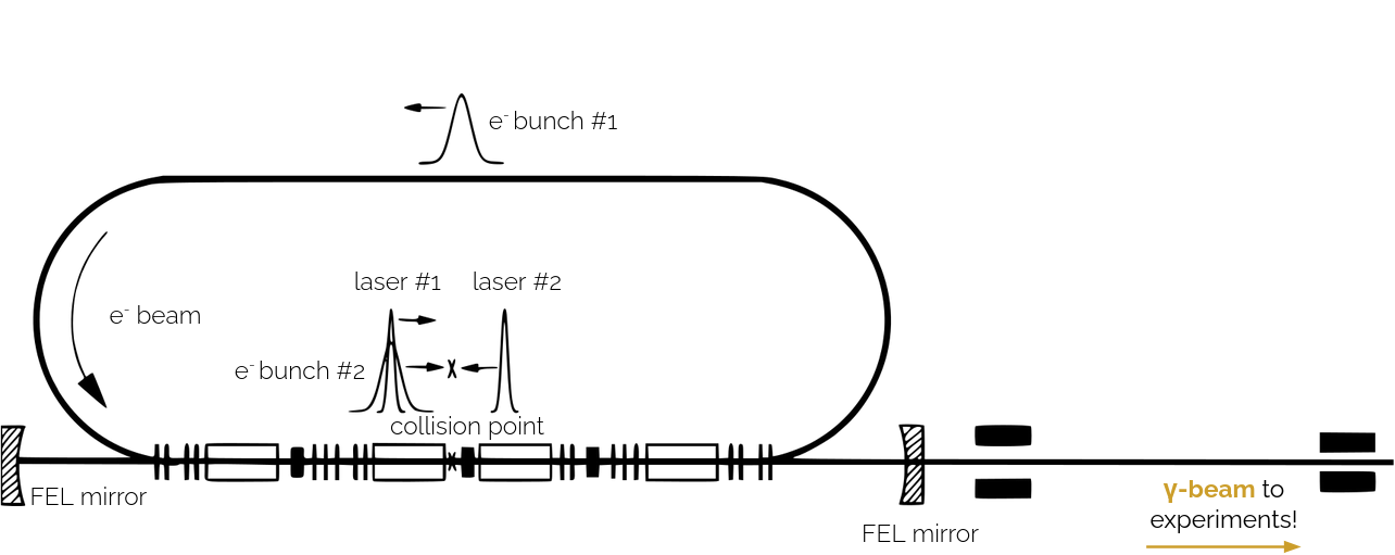
Compton backscattering: A low-energy laser photon is scattered off a relativistic electron beam. By tuning the electron energy and collision geometry, one can produce nearly monochromatic photons via the Compton formula: \begin{equation} E_\gamma = E_e \left(1 - \cos\theta\right) \frac{2E_\mathrm{laser}}{m_e c^2} / \left[1 + \frac{2E_e}{m_e c^2}(1-\cos\theta)\right] \end{equation}
Advantages:
- Excellent energy resolution (< 1% FWHM)
- Tunable beam energy by adjusting electron energy
- Narrow energy spread allows threshold measurements
Disadvantages:
- More complex infrastructure (linac + laser + collision geometry)
- Lower absolute photon flux compared to bremsstrahlung
- Higher operational cost
Major $\gamma$-ray beam facilities worldwide
The following table summarizes the key facilities used for photonuclear research in astrophysics:
| Facility | Country | Energy Range (MeV) | Flux ($\gamma$/s) | $\Delta E/E$ (FWHM) | Polarization | Technique |
|---|---|---|---|---|---|---|
| HI$\gamma$S (TUNL) | USA | 1–100 | $\leq 3 \times 10^{10}$ | 3–5% | Linear/Circular | Compton backscattering |
| ELI-NP | Romania | 0.2–19.5 | $\sim 2 \times 10^{8}$ | $\leq$0.5% | Linear | Laser Compton Scattering |
| NewSUBARU | Japan | 1–35 | $\sim 10^{7}$–$10^{8}$ | $\sim$3% | Linear/Pol. | Laser Compton Scattering |
| S-DALINAC | Germany | 5–70 | $10^{10}$–$10^{12}$ (integrated) | ~100% (broad) | Unpolarized | Bremsstrahlung |
The choice of facility depends on the physics questions:
- High flux, broad energy range: S-DALINAC or HI$\gamma$S for measuring integrated cross sections
- Excellent energy resolution: ELI-NP for threshold measurements and nuclear resonance fluorescence (NRF)
- Polarization studies: HI$\gamma$S for studying angular distributions and multipole decomposition
Detectors and Observables
To extract astrophysical information from $\gamma$-beam experiments, we need to measure:
-
Photonuclear cross sections $\sigma(E_\gamma)$ as a function of energy: Direct measurement of the reaction probability is the primary goal. By scanning the $\gamma$ energy across the relevant range (typically MeV–tens of MeV), one can identify resonances and measure threshold behavior. For the $\gamma$-process, typical threshold energies are 5–20 MeV (corresponding to the negative Q-values)
. -
Particle detection: The outgoing nuclei and/or neutrons from $(\gamma,n)$, $(\gamma,p)$, and $(\gamma,\alpha)$ reactions must be detected with:
- Silicon detectors for charged particles: Excellent energy and position resolution; provides particle identification via $\Delta E$–$E$ techniques
- Neutron detectors: Scintillators or time-projection chambers (TPCs) for measuring neutron energies and multiplicities
- CdZnTe or similar: Fast timing for coincidence measurements to identify multi-nucleon ejection
-
Angular distributions $\frac{d\sigma}{d\Omega}$: The angular distribution of outgoing particles constrains the multipolarity (E1, E2, M1, etc.) of the $\gamma$-ray interaction. This provides nuclear structure information beyond just the cross section magnitude
. -
Nuclear resonance fluorescence (NRF):
When a $\gamma$ ray elastically scatters off a nucleus, it reveals the position and width of excited states. NRF is particularly useful for identifying low-lying resonances that feed the ground state
; this is crucial for understanding stellar enhancement factors.
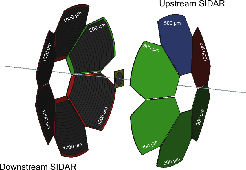
Example: The SIDAR array at HIγS
Case study- $^{102}$Pd+$\gamma$ at HI$\gamma$S (TUNL)
Why $^{102}$Pd?
$^{102}$Pd is one of the ~35 p-nuclei and plays a crucial role in $\gamma$-process nucleosynthesis for several reasons: At this nucleus, the reaction flow branches between $(\gamma,n)$ leading to $^{101}$Pd and $(\gamma,p)$ leading to $^{101}$Rh (or $(\gamma,\alpha)$). The competition between these two channels directly affects whether the reaction flow continues to lighter p-nuclei or remains in the Pd isotope chain.
The solar system abundances of light p-nuclei (including Pd and Rh isotopes) are difficult to reproduce with standard $\gamma$-process models. Understanding the branching at $^{102}$Pd is essential for solving this discrepancy.
The ($\gamma,p$) reaction to $^{101}$Rh has $Q = -7.81$ MeV (endothermic). This threshold is within the energy range of modern $\gamma$-beam facilities like HIγS (up to 100 MeV), making direct measurements feasible.
$^{102}$Pd is a stable nucleus with a long half-life, so it can be produced as a pure target without complications from radioactive decay.
Astrophysical relevance: In core-collapse supernovae, $^{102}$Pd experiences peak temperatures of ~2.5–3 GK. At these temperatures, the thermal population of excited states in $^{102}$Pd affects the branching ratio. Direct measurements constrain the ground-state contribution, which can then be extrapolated to excited states using nuclear models.
Experimental setup
The recent $^{102}$Pd$(\gamma,x)$ experiment (where x = p and α) at HIγS utilized:
-
$\gamma$-ray beam: Monochromatic, collimated beam produced via Compton backscattering. The beam is scanned from slightly above the threshold (~10 MeV) up to ~19 MeV to map out the excitation function.
-
Target: A thin $^{102}$Pd 78% enriched target (1.8 mg/cm$^2$ thickness) positioned at the center of the detector array.
-
Silicon Detector Array (SIDAR):
- Multiple silicon detectors arranged in rings around the target (~38% of 4π coverage)
- Measures the energy and angle of outgoing protons and alpha particles
- Energy resolution: ~100 keV (dominated by target thickness)
- Angular resolution: ~2.5° (allows extraction of angular distributions if desired)
-
Detector logic: A charged particle is identified by:
- Its energy loss in the silicon ($dE/dx$, related to charge and mass)
- Its residual energy after passing through the detector
- The combination determines whether it’s a proton, alpha, or heavier fragment
Measured quantities:
- Differential cross section $\frac{d\sigma}{dE_\gamma}$ for ($\gamma,p$) and ($\gamma,\alpha$) as functions of $E_\gamma$
- Angular distributions $\frac{d\sigma}{d\Omega}$ (if measured with sufficient angular resolution)
- Total $\gamma$-induced reaction cross sections by integrating over angles
Model expectations
Before the experiment, theoretical predictions (using TALYS) made specific predictions for the cross sections. The predictions depended on the choice of nuclear physics inputs that we discussed previously (OMP, $\gamma$SF and NLD).
Typical HF predictions:
- ($\gamma,p$) cross section: ~1–10 mb near 10 MeV above threshold
- ($\gamma,\alpha$) cross section: Smaller (~0.1–1 mb) but non-negligible
Uncertainties: HF predictions for this nucleus carry typical uncertainties of factors of 2–3 (sometimes more) due to the nuclear physics inputs. This is why direct measurements are essential.
Results and interpretation
The experimental data (provided in the companion notebook as pd102gp.dat) show the ($\gamma,p$) cross section as a function of $\gamma$-energy. Key observations include the threshold behavior, the energy dependance and its comparison with the the HF predictions. The cross section rises sharply above the 7.81 MeV threshold, reaching peak values of a few millibarns at ~10 MeV. The opening of the neutron channel at ~10.5 MeV is not as pronounced as expercted. Above ~15 MeV, the cross section behavior seems to flatten out. We can now use the measured cross sections to constrain the HF model inputs. If the measurement differs from theory, it suggests that one or more of the OMP, GSF, or NLD parameters needs refinement.
How does this feed back to nucleosynthesis?
Using the measured cross section $\sigma(E_\gamma)$ and detailed balance, one can calculate the stellar reaction rate:
\begin{equation} \lambda_\gamma = \frac{8\pi}{h^3 c^2}\int_0^\infty \frac{E_\gamma^2}{e^{E_\gamma/(kT)}-1} \sigma(E_\gamma) \, dE_\gamma \end{equation}
This integral weights the cross section by the thermal photon distribution (Planck function). At high stellar temperatures (T = 2–3 GK, relevant for the $\gamma$-process), the Planck function shifts weight to higher energies, emphasizing the cross section above ~15 MeV.
The updated rates, combined with the competing ($\gamma,n$) rates, determine the branching ratio in the astrophysical environment. This directly predicts the final abundance of $^{101}$Rh vs. the flux of nuclei progressing toward lighter p-nuclei. The notebook guides you through this calculation step by step.
Broader implications and open questions
Key open questions in the γ-process
-
Light p-nuclei discrepancy: Standard $\gamma$-process calculations struggle to reproduce the observed abundances of light p-nuclei (A ~ 90–120). This may indicate:
- Missing physics in the supernova models (e.g., rotation, magnetic fields, 3D effects)
- Contributions from alternative sites (e.g., C–O shell mergers, νp-process)
- Systematic uncertainties in nuclear reaction rates that haven’t been fully explored
-
Role of excited-state contributions: Most direct measurements target ground states. The contribution of excited states at astrophysical temperatures remains poorly constrained.
-
The importance of (γ,α) reactions: While ($\gamma,n$) dominates the reaction flow, ($\gamma,\alpha$) channels can open up new reaction paths or suppress certain isotopes. Precise measurements of ($\gamma,\alpha$) cross sections are still lacking for many nuclei.
-
Rare isotope beams: Many reaction for the $\gamma$-process involve unstable isotopes. Next-generation facilities (e.g., FRIB, GSI-FAIR) have very recently started to perform experiments on radioactive beams, allowing direct measurements on unstable nuclei
.
Future perspectives
Some ideas about the future directions in our field regarding the $\gamma$-process:
-
New generation of $\gamma$-ray sources:
- Higher intensity beams (increased flux by orders of magnitude)
- Improved energy resolution for better threshold studies
- Wider energy ranges to probe different astrophysical regimes
- Improved polarization capabilities for nuclear structure studies
-
Advanced detector technologies:
- Fast, large-volume TPCs for neutron detection and energy reconstruction
- $\gamma$-ray spectrometers for coincident photon detection
-
Collaboration with astrophysical observations:
- Solar abundances still set strong constraints on nucleosynthesis models
- Meteoritic data (presolar grains, isotope anomalies) provide complementary evidence
- Astronomical observations (s-process abundances in AGB stars, r-process signatures in neutron star mergers)
-
Bridging theory and experiment:
- Uncertainty quantification to propagate nuclear physics uncertainties through nucleosynthesis
- Bayesian approaches to constraining reaction rates from multiple experimental inputs
- Integrated frameworks combining nuclear physics, hydrodynamics, and observational constraints
Conclusions
The $\gamma$-process remains a fundamental open problem in nuclear astrophysics. Understanding where the p-nuclei come from requires inputs from different perspectives: state-of-the-art astrophysical modeling, careful nuclear measurements with $\gamma$-beams (or capture reactions), and theoretical nuclear physics to extrapolate beyond what we can measure. Each piece contributes to piecing together this complex cosmic puzzle.
Feel free to play with the companion notebook and get some hands-on experience with the data analysis and calculations that lie at the heart of this field. By working through the detailed balance calculations and rate conversions, you will gain insight into how laboratory measurements can help us understand the origin of the elements in the cosmos.