An introduction to thermonuclear reaction networks
Lecture notes for the 2nd Frontiers Summer School
What is a thermonuclear reaction network and why should I care?
If you work in nuclear astrophysics, you may not have realized the close connection between your work and thermonuclear reaction networks. Let us examine some examples:
- Student A works in low-energy experimental nuclear physics and she measured the cross section of an astrophysically interesting reaction for her dissertation,
- Postdoc B is an observational astronomer and has measured the elemental abundances of Galactic metal-poor stars,
- Student C works in nuclear theory and has implemented a new Equation of State (EoS) to be used in Neutron Star (NS) and Supernovae (SNe) simulations,
- Postdoc D wants to study the effect of a reaction rate to the energy generation in her hydrodynamics code.
What do they all have in common? Their results are interconnected using thermonuclear reaction networks!
Networks are groups of things that are connected in some way, and we can find them everywhere. The most common example is the social network: your family, friends, colleagues and the rest of the people you are interacting socially (nowadays we can find virtual counterparts of these networks). A network consists of nodes (in our social network example, people), and edges (social connections). There is a very active academic field which studies networks and their interactions, called network science.

Similarly, thermonuclear reaction networks connect nuclei via nuclear
processes, such as reactions and decays.
An additional complexity is that the reaction networks we will study in this
lecture evolve over time, according to the thermodynamical conditions of the
environment (typically only temperature, $T(t)$ and density, $\rho(t)$), and for this
reason we are also interested in the reactive flows.
In this lecture we will discuss how these reactions enter the network, when they matter and when they don’t.
We call these reactions thermonuclear because they are caused by the thermal motion
of the involved nuclei, which almost always obey a Maxwellian
distribution

A thermonuclear reaction network
is a system of first-order coupled differential equations,
which describes the abundance evolution and energy generation, and depends
only on the nuclear reaction rates and the local thermodynamical conditions
Thermonuclear reaction rates
Before we delve into the inner workings of thermonuclear reaction networks, let us first imagine that we are around 150 million kilometers (93 million miles) away from the Earth, inside the core of our beloved Sun. To enjoy the heat and warmth the Sun provides, there is an active transformation of its main ingredient, hydrogen (which also happens to be the most abundant element in the universe), to helium (the second most abundant element). From the small mass difference between $\mathrm{^1H} (p)$ and $\mathrm{^{4}He} (\alpha)$ there is a release of energy equal to:
\[\mathrm{Q = 4 \Delta m_{H} - \Delta m_{He} = 4 \cdot (7288.97~keV) - (2424.92~keV) = 26.731~MeV}\]where $\Delta m$ are the “mass excesses” of hydrogen and
helium
For the last 4.6 billion years hydrogen is continuously “burned” into helium
in the heart of the Sun. To familiarize ourselves with thermonuclear reaction networks,
we will recreate the main fusion process that powers the Sun, the proton-proton (pp-)
chain

Let us consider for simplicity that the core of the Sun is made out of only
four nuclear species, namely $\mathrm{^1H}~(p)$, $\mathrm{^2H}~(d)$, $\mathrm{^3He}$
and $\mathrm{^4He}~(\alpha)$
From now on, we will use the typical nuclear physics notation for nuclear reactions: $p(p,e^+ \nu_e)d$, $d(p,\gamma)\mathrm{^3He}$ and $\mathrm{^3He}(\mathrm{^3He},2p)\mathrm{^4He}$, respectively. The net effect in the environment is the conversion of 4 protons to one helium nucleus and the release of 26.73 MeV in the environment in the form of $\gamma$-rays and neutrinos. In the Figure below, you can see a visualization of the pp-chain in a pure $p$ gas.

These thermonuclear reactions have a twofold importance for astrophysical environments: first they generate energy that stabilizes the star from gravitational collapse and at the same time they transform its constituents by synthesizing new nuclear species.
The first step in the pp-chain is the $p(p,e^+ \nu_e)d$ reaction, in which a
proton is converted into a neutron, which becomes part of the deuteron. This
reaction is affected by the weak nuclear force, and for this reason its cross
section (or the probability that the reaction occurs in the stellar gas) is
very small. In fact, it is extremely difficult to recreate it in a laboratory,
due to the tiny event rate
The second step in the pp-chain is the $d(p,\gamma)\mathrm{^3He}$
reaction, where the deuteron was synthesized by the $p(p,e^+ \nu_e)d$
reaction. Reactions that emit a $\gamma$-ray in the exit channel are generally
called radiative capture reactions and are very common in nuclear
astrophysics
\begin{equation}\label{eq:1} r_{dp} = n_d n_p \langle \sigma v \rangle_{dp} = n_d n_p \int \sigma(v)~P(v)~v~dv \end{equation}
where $n_d$ and $n_p$ are the concentrations, or number densities, of $p$ and $d$ per unit volume (usually expressed in cm-3). These are dynamical quantities regulated by the nuclear processes that involve them. $\langle \sigma v \rangle_{dp}$ is the average value of the reaction cross section $\sigma$ (usually expressed in barns, where 1 b $\equiv$ 10-24 cm2) and the relative velocity distribution of the interacting particles.
Number density can change if the gas expands or contracts (remember that it is species per unit volume). For this reason, we need a conserved quantity which reflects the nuclear transformations that occur in the gas. There are two such quantities that are commonly used in astrophysics, the mass fraction, $X_i$ and the abundance, $Y_i$. The three quantities, number density, mass fraction and abundance are related through the following expression
\begin{equation}\label{eq:2} n_i = \frac{\rho N_A X_i}{A_i} = \rho N_A Y_i \end{equation}
where $A_i$ is the atomic mass of species $i$ in amu (for example $A_{\mathrm{^{4}He}}$= 4.0026 amu) and $N_A$ is the Avogadro constant ($N_A = 6.022 \times 10^{23}$ mol-1).
If we apply the nucleon number conservation in the
environment
\begin{equation}\label{eq:3} \sum_i X_i = 1 \end{equation}
\begin{equation}\label{eq:4} \sum_i A_i Y_i = 1 \end{equation}
Now that we have convinced ourselves that we are measuring the change of the constituents of the gas that is caused by nuclear processes, we can move on to the calculation of the thermonuclear reaction rate $\langle \sigma v \rangle$.
In a stellar gas, like in our example, the temperature is high enough to ionize completely the constituent atoms (bare nuclei), such that they do not experience any long range electronic interactions. The relative velocity of the interacting particles can be described by the Maxwell-Boltzmann distribution
\begin{equation}\label{eq:5} P(v) dv = \left( \frac{\mu}{2\pi kT} \right)^{3/2} e^{-\mu v^2/(2kT)} 4\pi v^2 dv \end{equation}
which expresses the probability that the relative velocity of two particles lies between $v$ and $v+dv$. $\mu = m_d m_p/ (m_d+m_p)$ is the reduced mass of the system, $k$ is the Boltzmann constant, with a value of $k= 8.6173 \times 10^{-5}$ eV/K and T is the gas temperature expressed in Kelvin. The Maxwell-Boltzmann distribution shows the following behavior: it increases linearly with energy E at low energies, E $\ll$ kT, reaches a maximum value at E = kT and decreases exponentially at high energies, E $\gg$ kT. This behavior is crucial when considering at which energies the astrophysically interesting reactions take place.
We can express the Maxwell-Boltzmann particle velocity distribution as an energy distribution (convert using $E= \frac{1}{2} \mu v^2$) and obtain the reaction rate in the center-of-mass energy (in units of cm3 mol-1 s-1)
\begin{equation}\label{eq:6} \langle \sigma v \rangle = \left( \frac{8}{\pi \mu}\right)^{1/2} (kT)^{-3/2} \int_0^\infty \sigma(E)~E~e^{-E/kT} dE \end{equation}
Equation \ref{eq:6} is a general expression for the thermonuclear reaction rate. In principle, the only missing piece for its calculation is the energy–dependent reaction cross section, $\sigma(E)$. Once this quantity is either measured experimentally, or estimated theoretically, It can then be integrated numerically and evaluated at the temperature of interest.
In general, there are few cases in which Equation \ref{eq:6} can be solved
analytically, because the cross section has a relatively simple energy
dependence. A smooth (non-resonant) and a strong (resonant) energy dependence
of the cross-section are encountered frequently in nuclear astrophysics
For non-resonant reactions, the cross section $\sigma(E)$ can be re-written as \begin{equation}\label{eq:7} \sigma(E) = \frac{S(E)}{E} e^{-2\pi \eta} \end{equation}
where $S(E)$ is called the astrophysical S-factor and it is a slowly varying function of energy that removes the strong $1/E$ energy dependence of $\sigma(E)$. Substituting Equation \ref{eq:7} to \ref{eq:6} gives us
\begin{equation}\label{eq:8} \langle \sigma v \rangle = \left(\frac{8}{\pi \mu}\right)^{1/2} (kT)^{-3/2} \int_0^\infty S(E) e^{-2\pi \eta} e^{-E/KT} dE \end{equation}
The integrant of the above expression exhibits a very interesting energy dependence. Multiplying the transmission probability through the Coulomb barrier, $e^{-2\pi \eta}$, which increases with increasing energy, with the Maxwell-Boltzmann factor, which decreases with increasing energy, results in a peak which defines an energy region where it is more probable for nuclear reactions to occur in a stellar gas. The peak is commonly referred to as the Gamow peak.
For resonant reactions, the cross section can be described by the single-level
Breit-Wigner formula
\begin{equation}\label{eq:9} \sigma(E) = \frac{\lambda}{4\pi} \frac{(2J+1)}{(2j_a+1)(2j_b+1)} (1+\delta_{ab}) \frac{\Gamma_1(E) \Gamma_2(E)}{(E_r-E)^2+(\Gamma(E)/2)^2} \end{equation}
where $\lambda$ is the de Broglie wavelength, which expresses the wave nature of the interacting particles, $j_i$ are the spin of projectile and target, $J$ and $E_r$ are the spin and energy of the resonance respectively, $Γ_i$ are the partial widths for entrance and exit channels and $\Gamma$ is the sum of all the partial widths $\Gamma_i$, which correspond to the energetically allowed decay channels.
Using Equation \ref{eq:9} we can solve analytically Equation \ref{eq:6}. In the case of many resonances, we can add them incoherently and write the thermonuclear reaction rate as follows \begin{equation}\label{eq:10} \langle \sigma v \rangle = \left(\frac{2\pi}{\mu kT}\right)^{3/2} \hbar^2 \sum_i (\omega \gamma)_i e^{-E_i/kT} \end{equation}
where $\omega = (2J+1)/(2j_a+1)(2j_b+1)$ is the nuclear spin factor and $\omega \gamma$ is called the resonance strength, $\omega \gamma \equiv \omega \frac{\Gamma_1 \Gamma_2}{\Gamma}$, and it is proportional to the area under the resonance cross section, or the product of the total resonance width and the cross section at the resonance energy, $\Gamma \cdot \sigma(E=E_r)$.
Another way to calculate the reaction cross section $\sigma(E)$ or the astrophysical S-factor is the use of R-matrix theory.
See R.J. deBoer lecture
The main assumption of that framework is that the particle configuration space can be separated in an
internal region, where the total wave function can be expanded into a complete
set of eigenstates and the external where the possible combinations of
particles exist
For nucleosynthesis processes that involve exotic nuclei, reaction rates are usually based on theoretical estimates for $\sigma(E)$. For example, in the $r$-process we rely on calculations based on the Hauser-Feshbach statistical model for the $(n, \gamma)$ reactions on exotic neutron-rich species.
See G. Perdikakis lecture
This model is used to describe cross sections in higher excitation energies of intermediate and heavy nuclei, where the density of nuclear levels is high enough to take a statistically average contribution of many Breit-Wigner resonances. It assumes that the compound nucleus formed in a reaction undergoes a sequence of statistical decays, where the excitation energy is partitioned among the available degrees of freedom of the system, such as nucleons, $\gamma$-rays, and other particles.
To calculate thermonuclear reaction rates, one needs to solve Equation
\ref{eq:6} numerically or analytically. Given that reaction rates carry
uncertainty from many different factors, such as resonance energies, resonance
strengths etc., we need a statistically meaningful way to treat them. One
of the ways used in the nuclear astrophysics community is to treat each
nuclear physics input as a (lognormal) distribution and sample thousands of
times using a Monte Carlo technique, solving Equation \ref{eq:6} every time.
That way, one calculates a thermonuclear reaction rate with temperature dependent uncertainty
(essentially for every temperature point, you get a distribution for the
reaction rate, and from the 16th (lower) and 84th (high) percentile you can
define the $1\sigma$ confidence level). The code RatesMC, which was
developed by R. Longland (NCSU/TUNL) performs such
calculations.
More recently, Bayesian statistics along with Markov Chain Monte Carlo (MCMC)
algorithms have been used to calculate S-factors of astrophysically important
reactions
Forming the network
The rate equations
Let us return to the core of the Sun and try to write the differential equations that describe the abundance evolution for all the different species. $p$ is destroyed by the $p(p,e^+\nu)d$ and $d(p,\gamma)\mathrm{^{3}He}$ reactions and produced by the $\mathrm{^3He(^3He, 2p)^4He}$. We expect that this will be proportional to the initial abundance and also the reaction rate. Using Equations \ref{eq:1} and \ref{eq:2} we can write
\begin{equation}\label{abu:p} \frac{dY_p}{dt} = - \rho N_A Y_p^2 \langle \sigma v \rangle_{pp} - \rho N_A Y_d Y_p \langle \sigma v \rangle_{dp} + \rho N_A Y_{\mathrm{^3He}}^2 \langle \sigma v \rangle_{\mathrm{^3He}\mathrm{^3He}} \end{equation}
Similarly, $d$ is produced by the $p(p,e^+\nu)d$ and destroyed by the $d(p,\gamma)\mathrm{^{3}He}$.
\begin{equation}\label{abu:d} \frac{dY_d}{dt} = \rho N_A \frac{Y_p^2}{2} \langle \sigma v \rangle_{pp} - \rho N_A Y_d Y_p \langle \sigma v \rangle_{dp} \end{equation}
$\mathrm{^3He}$ is created by the $d(p,\gamma)\mathrm{^{3}He}$ and destroyed by the $\mathrm{^{3}He}(\mathrm{^{3}He},2p)\mathrm{^{4}He}$:
\begin{equation}\label{abu:3he} \frac{dY_{\mathrm{^3He}}}{dt} = \rho N_A Y_d Y_p \langle \sigma v \rangle_{dp} - \rho N_A Y_{\mathrm{^3He}}^2 \langle \sigma v \rangle_{\mathrm{^3He}\mathrm{^3He}} \end{equation}
Finally $\alpha$-particles are created only by the $\mathrm{^{3}He}(\mathrm{^{3}He},2p)\mathrm{^{4}He}$ reaction.
\begin{equation}\label{abu:he4} \frac{dY_\alpha}{dt} = \rho N_A \frac{Y_{\mathrm{^3He}}^2}{2} \langle \sigma v \rangle_{\mathrm{^3He ^3He}} \end{equation}
Imagine doing the same exercise for thousands of nuclei that are connected
with tens of thousands of reactions!
Most reactions can be grouped into three
functional categories, according to the number of interacting nuclei:
reactions involving a single species, such as decays and electron/positron
captures, two (e.g. our $p(d,\gamma)\mathrm{^3He}$) and three
(e.g. $\mathrm{^4He(\alpha \alpha,\gamma)^{12}C}$ – triple–$\alpha$
reaction) nuclei
where $\lambda_j$ is called the decay constant, $\langle \sigma v \rangle_{jk}$ and $\langle \sigma v \rangle_{jkl}$ are the thermonuclear reaction rates for 2- and 3-body reactions. Note that in the latter we multiplied by $(\rho N_A)^2$ to account for the third particle. The $N$s are used to make sure we do not double-count produced (or destroyed) species.
We can also express the same relation, more generally as \begin{equation}\label{eq:general} \dot{\mathbf{y}} = f(\mathbf{y}) \end{equation}
where $\mathbf{y}$ is the vector of all the abundances $Y_i$ (or mass fractions $X_i$) in the network ($Y_1$, $Y_2$, $\cdots$, $Y_{i_{max}}$), $\dot{\mathbf{y}}$ is the time derivative, and $f$ is a function which depends on the abundances $Y_i$ and the thermodynamical properties of the environment, $T(t), \rho(t), \ldots$.
The ingredients
To solve (integrate) the rate equation we need some input. First and foremost, we need the nuclear physics information about the isotopes in the network; that is their reaction rates, reaction Q-values, half-lifes (if they are radioactive), fission fragment distributions (if they are fissionable) and partition functions, the sum of thermally populated levels.
You might wonder why we did not mention nuclear masses, which have a high level of ongoing research activity. The nuclear masses enter the rate equation via the Q-value (for example in neutron captures, photodissociation rates and $\beta$-decays). If a new mass measurement is made, that updates the Q-value in the network.
See A. Kankainen and M. Li lectures
For example, in the $r$-process, $(n, \gamma)$ and $(\gamma, n)$ rates depend on the mass
difference, or neutron separation energy $S_n$. Specifically for the
$(\gamma, n)$ rates, using the principle of detailed balance and $S_n$ we can write
\begin{equation} \lambda_\gamma \propto T^{3/2} \exp\left[ -\frac{S_n(Z,N)}{kT} \right] \langle \sigma v \rangle_{(Z, N-1)} \end{equation}
where $\langle \sigma v \rangle_{(Z, N-1)}$ is the neutron capture - $(n, \gamma)$ - rate of the neighboring nucleus.
Another nuclear input that is used when solving a thermonuclear reaction network is the Equation Of State (EOS), which gives us the relation between temperature, pressure, and density in the gas.
As far as the astrophysics input is concerned we are mainly interested in the time evolution of the temperature and density of the plasma and in many cases its electron mole fraction $Y_e \equiv n_p (n_p+n_n)^{-1}$. If $Y_e < 0.5$ we have a neutron-rich gas, and in the case of $Y_e>0.5$ we have a neutron-deficient one. In some special cases, where the neutrino properties are of interest (e.g. in neutrino-driven wind ejecta) we also need to know the evolution of neutrino-related quantities, such as their luminosity, which are used to calculate the $Y_e$.
The properties of the astrophysical environment can be obtained from hydrodynamic
simulations. For quiescent, hydrostatic burning (e.g. hydrogen burning in a
main sequence star) the temperature and density history of the gas is constant
and the local energy release from nuclear reactions does not change the conditions.
For other processes, however, such that in explosive nucleosynthesis we need
to know the time evolution of the thermodynamical quantities. In cases where
there is a shock which heats up and compresses the gas to a peak temperature
and density and then expands adiabatically, we can easily model it using an
exponential function $T(t) = T_{peak}e^{-T/\tau_T}, \rho(t)= \rho_{peak}e^{-t/\tau_\rho}$.
These are also known as “parametric profiles”, since we can change the main
parameters of each relation (peak value and the timescale). The advantage of
such a paramtrization is that it is computationally less expensive and it also
allows for the exploration of the relevant parameter phase space (see for example the work of
Iliadis et al (2018)
Solving the network
In the previous sections we constructed the system of differential equations that describes the time evolution of the abundances and we know the initial conditions of the system (in our solar burning example is $X_p(t=0)=1, X_d=X_{\mathrm{^3He}}=X_\alpha=0$). We are now ready to solve (integrate) the rate equations.
The coefficients of our rate equations (thermonuclear reaction rates) span many orders of magnitude, due to their strong temperature dependence (Equation \ref{eq:6}). For example, in the pp-chain network, the $p(p,e^+\nu)d$ reaction has a timescale of billions of years, and the $\mathrm{p(d,\gamma)^3He}$ only seconds! For this reason, our system is stiff, meaning that its solution is numerically unstable, and as such, smaller steps of integration must be used.
Let us examine an example of a stiff equation:
\begin{equation}\label{eq:stiff} \dot{x} = -21 x(t) + e^{-t} \end{equation}
with boundary condition \(x(0) = 0\). Below you can find a python
script which solves the equation and also shows the size of the timesteps used.

The above equation is considered stiff because the solution has rapidly changing behavior on a short timescale (due to the exponential term $e^{-t}$), but the overall behavior of the solution changes much more slowly (due to the negative coefficient on $y$). This can make it difficult to solve numerically using standard methods, as the step size must be very small to capture the fast changes accurately (as in for $t \ll 1$).
If we return to our general equation for the network (Equation \ref{eq:general}) we can approximate the time derivative by a finite difference
\begin{equation} \mathbf{\dot{y}_n} = \frac{\mathbf{y_{n+1}} - \mathbf{y_n}}{h} = (1-\Theta) \mathbf{\dot{y}}_{n+1} + \Theta \mathbf{\dot{y}}_n \end{equation}
where $\mathbf{y_n}, \mathbf{y_{n+1}}$ are the abundance vectors in time $t_n$ and $t_{n+1}$, and $h$ is the integration time-step. According to the choice of $\Theta$ we get different integration methods
\[\frac{\mathbf{y_{n+1}} - \mathbf{y_n}}{h} = \begin{cases} \mathbf{\dot{y}_n} & \Theta=1,~\text{explicit forward} \\ \frac{1}{2}[\mathbf{\dot{y}_{n+1}} + \mathbf{\dot{y}_n}] & \Theta= 1/2,~\text{semi-implicit trapezoidal} \\ \mathbf{\dot{y}_{n+1}} & \Theta=0,~\text{implicit backwards} \end{cases}\]The explicit scheme will encounter difficulties due to the stiffness of the problem, since the integration time steps will have to become tiny. Using an implicit scheme, we can express the change in abundances using Equation \ref{eq:general} as
\begin{equation}\label{eq:implicit} \mathbf{y_{n+1}} = \mathbf{y_n} + h f(t_{n+1}, \mathbf{y}, \ldots) \end{equation}
Thermonuclear reaction network codes employ backwards/implicit or semi-implicit methods, due to the stiffness
of the nucleosynthesis reaction networks. Widely
used examples include “Wagoner’s method” (2nd order Runge-Kutta)
Generaly, to find a solution of Equation \ref{eq:implicit} we can re-write it in a matrix form as follows \begin{equation}\label{eq:jacobian} [\mathbf{I}- h \mathbf{J}]\mathbf{y_{n+1}} = \mathbf{y_n} \end{equation}
$\mathbf{I}$ is the unitary matrix and $\mathbf{J} = \partial f / \partial \mathbf{y}$ is called the Jacobian matrix.
The Jacobian matrix
We can write the Jacobian $\mathbf{J}$ in its matrix form
\[\mathbf{J}(Y_1, \ldots, Y_n)= \begin{vmatrix} \frac{\partial \dot{Y_1}}{\partial Y_1} & \ldots & \frac{\partial \dot{Y_1}}{\partial Y_{i_{max}}} \\ \vdots & \ddots & \vdots \\ \frac{\partial \dot{Y}_{i_{max}}}{\partial Y_1} & \ldots & \frac{\partial \dot{Y}_{i_{max}}}{\partial Y_{i_{max}}}\end{vmatrix}\]Note that we are taking the partial derivative of individual abundances $Y_i$ in each matrix element. The resulting Jacobian’s size is $n_{max} \times n_{max}$. For our pp-chain example, if we make the substitution $R_{ab} = \rho N_A \langle \sigma v \rangle_{ab}$, the Jacobian takes the following form
\[\mathcal{J}= \begin{vmatrix} -2Y_p R_{pp} - Y_d R_{pd} & - Y_p R_{dp} & 2 Y_{\mathrm{^3He}} R_{\mathrm{^3He^3He}} & 0 \\ Y_p R_{pp} - Y_d R_{dp} & -Y_p R_{dp} & 0 & 0 \\ Y_d R_{dp} & Y_p R_{dp} & -2Y_{\mathrm{^3He}}R_{\mathrm{^3He^3He}} & 0 \\ 0 & 0 & Y_{\mathrm{^3He}} R_{\mathrm{^3He ^3He}} & 0 \end{vmatrix}\]Each Jacobian matrix element represents the flow of an isotope (positive or negative) per second.
A more mathematically rigorous definition of the stiffness of a reaction
network states that the negative $\mathcal{R}(\lambda_j)$ (the real
part of the Jacobian eigenvalues $\lambda_j$)
for $j = 1,2,\ldots, N$. In the thermonuclear reaction networks $\mathcal{S} > 10^{15}$ are typical, due to the orders of magnitude differences in the reaction rates. The number of zero entries in the Jacobian (sparcity) increases with increasing number of isotopes in the network.
With a few exceptions (e.g. $\mathrm{^{12}C+^{12}C, ^{12}C+^{16}O, 3\alpha}$ or fission) for each nucleus we only have to consider reactions linking it to the nearby species by the capture of a proton, neutron, helium nucleus or $\gamma$-ray and their reverse. That is 12 different reaction types, namely $(p,\gamma)$, $(\alpha, p)$, $(p,n)$, $(\alpha, \gamma)$, $(\alpha, n)$, $(n,\gamma)$, $(n,p)$, $(\gamma, p)$, $(n, \alpha)$, $(\gamma, \alpha)$, $(p, \alpha)$ and $(\gamma, n)$.

The solvers
The most computationally intensive part of a thermonuclear reaction network calculation is solving Equation \ref{eq:jacobian}. Dedicated sparse solvers are used to perform this operation and below you can find a short list of the most commonly used ones
The pp-chain abundances
If we solve the reaction network using any of the methods we discussed above, we can get the time evolution of the abundances (mass fractions) for the four species in the pp-chains.

If you look closely, there is an interesting feature in the evolution of $X_p$ and $X_d$.
A few special cases
In general we just need to solve the rate equation for every species in the network, however there are two special cases, where the abundance evolution can be calculated very easily.
Equilibrium
In the pp-chain example, starting with a pure proton gas, Equation \ref{abu:d} will only have the first term in the right-hand side. Gradually, the $p(p,e^+\nu_e)d$ reaction will produce deuteron, but it will also be destroyed by the $p(d,\gamma)\mathrm{^3He}$ reaction. Eventually the deuteron abundance will reach an equilibrium ($\frac{dY_d}{dt}=0$), meaning that its abundance will stay constant over time, despite the nuclear reactions that occur.
To find the equilibrium ratio between deuteron and protons, we just need to solve Equation \ref{abu:d}
\[\frac{dY_d}{dt} = 0 \rightarrow \frac{Y_d}{Y_p} = \frac{\langle \sigma v \rangle_{pp}}{2\langle \sigma v \rangle_{dp}}\]Even if we had a lot of deuteron in our stellar gas, the equilibrium would still be achieved. That is because the second term in Equation \ref{abu:d} will dominate in early times, destroying deuteron, until the equilibrium is established.
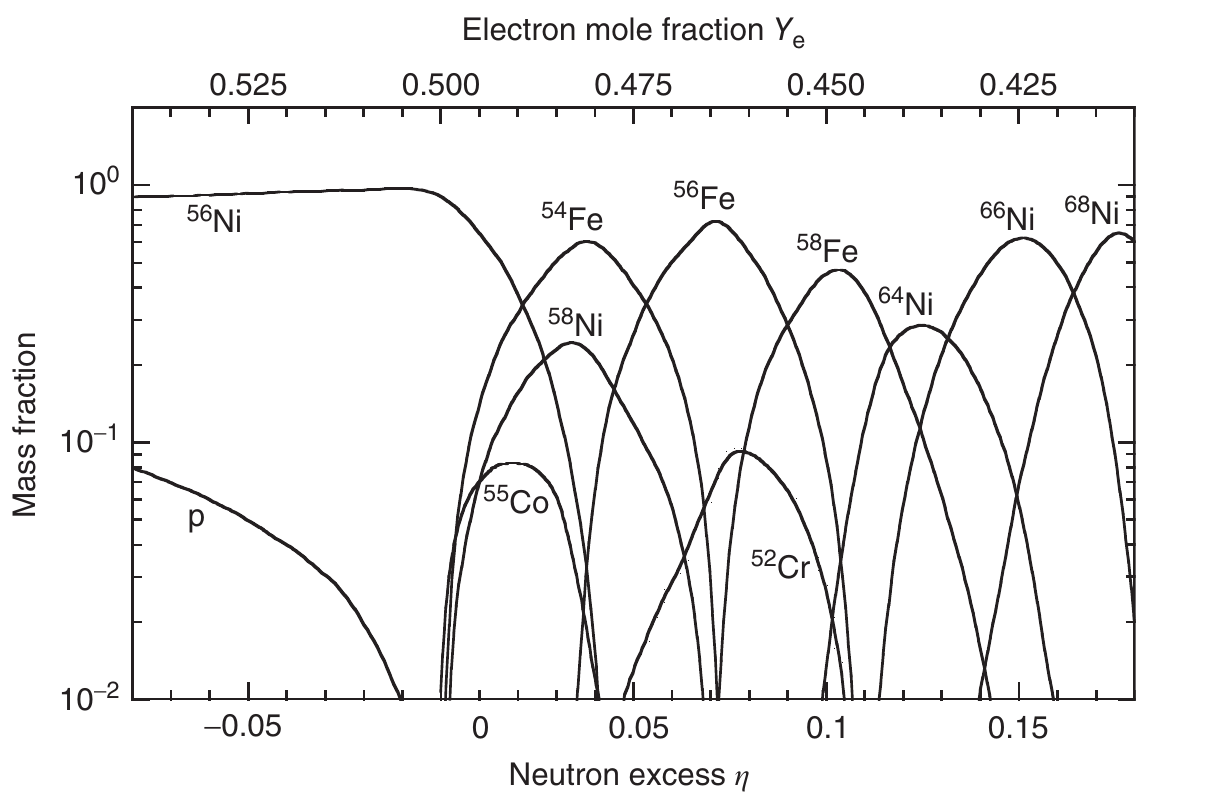
Nuclear Statistical Equilibrium (NSE)
Another special case occurs when the temperature in the astrophysical gas is very high ($T \geq 3 \times 10^9~K$). In such conditions, the thermonuclear reaction rates may be fast enough to achieve equilibrium faster than the timescale of the astophysical setting (in a core-collapse supernova or a neutron star merger, for example).
In this Nuclear Statistical Equilibrium (NSE), all nuclei are in balance through strong and electromagnetic interactions. At NSE conditions, the nuclear reaction network is greatly simplified and the abundance $Y_i$, of each species can be calculated in terms of the abundance of protons $Y_p$, and neutrons, $Y_n$, by applying the Saha equation
\begin{equation} Y_i = G_i \left(\rho N_A\right)^{A_i-1} \frac{A_i^{3/2}}{2_i^A} \left( \frac{2\pi \hbar^2}{m kT}\right)^{\frac{3}{2}(A_i-1)} e^{B_i/kT} Y_n^{N_i} Y_p^{Z_i} \end{equation}
where $G_i$ and $B_i$ is the partition function and binding energy of species $i$, $A_i$ is its mass number, $N$ the number of neutrons, $Z$ the number of protons and $\rho$ and $T$ are the density and temperature of the environment. In other words, in NSE the composition of the nuclear matter is determined by statistical mechanics alone and is independent of the previous nucleosynthesis history of the matter. The unique solution of the network for ($T,\rho,Y_e$) can be obtained using two constraints, namely mass (Equation \ref{eq:3} or \ref{eq:4}) and charge conservation
\begin{equation}\label{eq:0} \sum_i Z_i Y_i = Y_e \end{equation}
In the Figure below we can see how the most dominant species change as the neutron richness of the material changes for the same temperature and density (neutron excess $\eta \equiv \sum_i (A_i-2Z_i)Y_i$, where $A_i$ and $Z_i$ is the mass number and the number of protons for species $i$).
Energy generation
As we have already discussed, nuclear reactions release energy from the conversion of nucleons, and that affects the evolution of the astrophysical environment. The energy released by nuclear reactions and neutrinos, $\mathrm{\epsilon}$, can be calculated using
\begin{equation} \epsilon= - \sum_i N_A m_i c^2 \frac{dY_i}{dt}-\frac{d\epsilon_\nu}{dt}~\text{(MeV/g s}) \end{equation} where $m_i c^2$ is the rest mass energy of species $i$ in MeV and the last term in the right-hand side corresponds to the neutrino losses.
The following table shows the energy released from different burning
stages
| Process | Burning stage | q (MeV/nucleon) |
|---|---|---|
| $\mathrm{ H \rightarrow ^4He}$ | Hydrogen burning | 5-7 |
| $\mathrm{ 3\alpha \rightarrow ^{12}C}$ | Hydrogen burning | 0.606 |
| $\mathrm{ 4\alpha \rightarrow ^{16}O}$ | Helium burning | 0.902 |
| $\mathrm{ 2^{12}C \rightarrow ^{24}Mg}$ | Helium burning | 0.52 |
| $\mathrm{ 2^{20}Ne \rightarrow ^{16}O+^{24}Mg}$ | Neon burning | 0.11 |
| $\mathrm{ 2^{16}O \rightarrow ^{32}Si}$ | Oxygen burning | 0.52 |
| $\mathrm{ ^{28}Si \rightarrow ^{56}Ni}$ | Silicon burning | 0-0.31 |
Hydrodynamic codes require an accurate energy generation calculation, but
including thousands of species in the reaction network and solving stellar
evolution equations is computationally expensive.
For this reason, reduced networks are used instead, which include much less
species, but can follow the energy generation with a ~20% uncertainty. A typical
reaction network for hydrodynamic codes include $\alpha$-nuclei reaction network from He to Ni
$\mathrm{^4He}$, $\mathrm{^{12}C}$, $\mathrm{^{16}O}$, $\mathrm{^{20}Ne}$,
$\mathrm{^{24}Mg}$, $\mathrm{^{28}Si}$, $\mathrm{^{32}S}$, $\mathrm{^{36}Ar}$,
$\mathrm{^{40}Ca}$, $\mathrm{^{44}Ti}$, $\mathrm{^{48}Cr}$, $\mathrm{^{52}Fe}$
and $\mathrm{^{56}Ni}$ connected mainly by $(\alpha,\gamma)-(\gamma,\alpha)$
reactions, the triple-$\alpha$ reaction and the heavy ion reactions
$\mathrm{^{12}C+^{12}C}$, $\mathrm{^{12}C+^{16}O}$, and $\mathrm{^{16}O+^{16}O}$
The codes
After all this discussion about reaction networks, do you want to run some
calculations? That’s great! 😁 There are many codes in the nuclear
astrophysics community that are used for different nucleosynthesis processes;
some of them are open-source, others are not. I have compiled a
non-exhaustive list of such codes in the following table
Sensitivity studies using reaction networks
One of the awesome things we can do using thermonuclear reaction networks,
given the capabilities of modern computers, is multiple (>thousands)
calculations of the same profile (astrophysical condition). What can we learn
from that? By changing individual nuclear parameters, for example a reaction
rate, one can see the effect in the final elemental or even isotopic abundance
pattern. Through the years researchers in our field have taken different
approaches for these sensitivity studies. In the 2000s it was common to
vary individually reaction rates within their uncertainty: a typical example
is the seminal work of Iliadis et al. (2002)
During the 2010s researchers start using Monte Carlo (MC) algorithms to perform sensitivity studies. In this class of works - some notable examples for different nucleosynthesis scenarios are listed in the table below - reaction rates are randomly sampled from a distribution, which reflects their uncertainty, in every calculation. The reactions that influence abundances are identified by the correlation between the factor by which the rate was changed and the effect in the abundance.
| Scenario | Reference | Notes |
|---|---|---|
| BBN | Iliadis and Coc (2020) |
MC study using Bayesian rates |
| Nova nucleosynthesis | Iliadis et al (2002) |
Individual rates change |
| $s$-process | Cescutti et al. (2018) |
MC study |
| $i$-process | Denissenkov et al. (2021) |
MC study of $(n, \gamma)$ rates |
| weak $r$-process | Bliss et al. (2020) |
MC study of $(\alpha, n)$ rates |
| $\nu p$-process | Wanajo et al (2011) |
Individual rates, MC study |
| $r$-process | Mumpower et al. (2016) |
MC study on nuclear masses, β-decay halflives and $(n,\gamma)$ rates, fission barriers, MCMC for lanthanide production |
| $\gamma$-process | Rapp et al (2006) |
Individual rates change, MC study |
| $rp$-process | Parikh et al. (2008) |
Individual rates change |
| Type Ia nucleosynthesis | Parikh et al (2013) |
Individual rates change, MC study |
Take-home message
Combining everything we have discussed so far, a thermonuclear reaction network is a system of ordinary coupled differential equations (ODEs), which describes the abundance evolution ($\mathbf{y}$) and energy generation ($\epsilon$). The main input to solve the equations is provided by the nuclear reaction rates (except in the case of NSE) and the local thermodynamical conditions. The size of these networks can vary according to the astrophysical environment, with quiescent stellar burning, like the pp-chain, being much smaller compared to explosive burning ($r$-process). The main computationally expensive part of solving the network equations is to find the solution of Equation \ref{eq:jacobian} using the Jacobian matrix.
If there is one thing you should remember from this lecture, it is the following:
Nuclear reaction networks are an indispensable tool for a nuclear astrophysicist. Learn how it works and use it to your advantage!